Data Warehouse Modeling Techniques
In this article we will go over the big three approaches for modeling analytical data.
We will go through some definitions around data modeling and database design approaches as well as the differences between a data warehouse and a data mart, how they are used in business intelligence and data analytics and the modeling techniques applied with them.
So let’s get started!
Contents
- What is a Data Warehouse?
- Data Warehouse vs Data Mart
- What is Data Modeling?
- Normalization vs Denormalization
- Data Warehouse Modeling Techniques
- Modeling Techniques Implementation on Databricks Lakehouse Platform
- Recap
- Resources
What is a Data Warehouse?
Data Warehouse is not the same as a database but rather typically built on top of other databases. It aggregates data from dozens of data sources such as operational systems or external systems and the data is actually copied rather than moved.
Building a Data Warehouse serves the purpose of having a one stop shop: all your data in a single location which will enable you to make data driven decisions through trend analysis and business intelligence.
Data Warehouse vs Data Mart
Unlike the data warehouse which is a centralized data repository that provides a holistic view on the organization’s data, data mart is a specialized and focused subset of a data warehouse. It supports specific analytical needs and is generally easier and quicker to design and implement compared to a data warehouse.
What is Data Modeling?
Data Modeling is the process of creating a visual representation of a system’s data to represent it in an easy way for reusability, flexibility, and scalability. The output is usually a collection of living documents that evolve along with changes to business needs and serve the purpose of facilitating communication among stakeholders and the foundation for later database implementation and analysis.
The process of crafting data models involves 3 steps:
- Conceptual
- Analysis and design phase to understand the key business entities and attributes and capture their interactions as per the business processes and rules within the organization.
- Logical
- Technology agnostic model that adds more details and relations between entities for how the conceptual model will be implemented.
- Physical
- Defines how the logical model will be implemented using the system and technology in question to ensure that the writes and reads can be performed efficiently. It gives details about:
- Data field types as represented in the Database Management System (DBMS)
- Data relationships as represented in the DBMS
- Additional details, such as performance tuning
- Defines how the logical model will be implemented using the system and technology in question to ensure that the writes and reads can be performed efficiently. It gives details about:
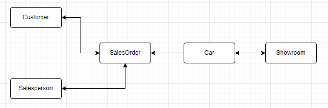
To better illustrate these steps, let’s consider an Auto Dealership as an example and model the potential system’s data. For instance, the diagram below highlights the different data entities and their relationships of the business on a conceptual level:
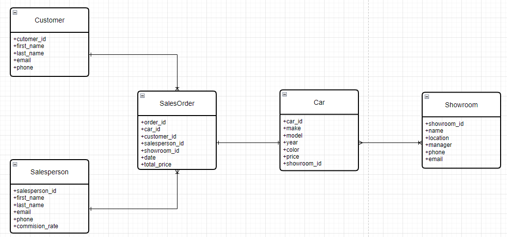
Adding more details to the identified entities will result in the following logical diagram:
Finally, the physical model will depend on the chosen database technology and will involve considerations such as how easy it is to manage it and will it be able to handle the load if the data volume scales.
Normalization vs Denormalization
Normalization and Denormalization are two opposing approaches to database design.
Normalization
In normalization, the focus is on reducing data redundancy and non-consistency and improving data integrity. This is achieved by organizing data into separate related tables in accordance with normal forms.
There are several normal forms each building upon the previous one and the main normalization norms are:
- First normal form (1NF)
- Each column is unique and has a single value. The table has a unique primary key.
- Second normal form (2NF)
- The requirements of 1NF, plus partial dependencies are removed.
- Third normal form (3NF)
- The requirements of 2NF, plus each table contains only relevant Fields related to its primary key and has no transitive dependencies.
A partial dependency occurs when a subset of fields in a composite key can be used to determine a non-key column of the table.
For example, considering the following table:
| StudentID | CourseID | StudentName | CourseName | InstructorName |
|---|---|---|---|---|
| 101 | CS101 | John | Database | Dr. Smith |
| 102 | CS102 | Emma | Networking | Dr. Johnson |
| 103 | CS102 | John | Networking | Dr. Johnson |
Table 1: Partial Dependency Example
- The primary key is the combination of (StudentId, CourseID)
- StudentName depends only on StudentID
- CourseName depends only on CourseID
- Here, we have two partial dependencies:
- StudentID → StudentName
- CourseID → CourseName
A transitive dependency occurs when a non-key field depends on another non-key field.
For example, considering the following table:
| EmployeeID | EmployeeName | DepartmentID | DepartmentName |
|---|---|---|---|
| E01 | Alice | D1 | Sales |
| E02 | Bob | D2 | Marketing |
| E03 | Charlie | D1 | Sales |
Table 2: Transitive Dependency Example
- The primary key is EmployeeID
- EmployeeName depends on EmployeeID
- DepartmentID depends on EmployeeID
- DepartmentName depends on DepartmentID
- Here, we have a transitive dependency:
- EmployeeID → DepartmentID → DepartmentName
Most practical database designs typically aim for 3NF as it generally provides a good balance between data integrity and performance.
In general, normalization is best suited for systems with frequent insert, update, and delete operations, like transactional databases. What about denormalization?
Denormalization
Denormalization on the other hand focuses on improving query performance, especially for read-heavy workloads, by combining related data from multiple tables increasing data redundancy and storage requirements and decreasing the number of tables in the database.
Denormalization is ideal for reporting systems and data warehouses where complex joins are expensive.
The choice between normalization and denormalization depends on specific application needs:
- Use normalization when data integrity and consistency are crucial, and when the database undergoes frequent updates.
- Opt for denormalization when query performance is a priority, especially for read-intensive applications or when complex joins significantly slow down data retrieval.
Data Warehouse Modeling Techniques
The three big approaches for modeling analytical data are:
- Inmon
- Top-down approach
- Advocates for creating a centralized, integrated Enterprise Data Warehouse (EDW)
- Uses a normalized structure (3NF) for the core warehouse where data is organized by subject reflecting the overall business structure
- Data Marts are created from the EDW as needed for analytical needs
- The popular option for modeling the data mart is a Star Schema
- Rules how to build data warehouse, store and organise data (Bill Inmon, 1990):
- Integrated = other data sources
- Subject oriented = reorganise the data per subject
- Time variant = data warehouse contains historical data
- Non volatile = data warehouse remains stable between refreshes
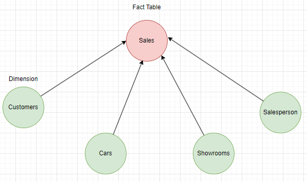
Continuing with the auto dealership example, an example of a star schema of the EDW is shown below:
- Kimball
- Bottom up approach
- Focuses on building data marts that address specific business processes making the data mart the data warehouse itself
- Uses a Star or Snowflake Schema for the design of the data marts
- Data is modulated with two general types of tables: Facts and Dimensions
- A slowly changing dimension (SCD) is necessary to track changes in dimensions
- SCD three most common ones:
- Type 1
- Overwrite existing dimension records. This is super simple and means you have no access to the deleted historical dimension records
- Type 2
- Keep a full history of dimension records. When a record changes, that specific record is flagged as changed, and a new dimension record is created that reflects the current status of the attributes
- Type 3
- A type 3 SCD is similar to a type 2 SCD, but instead of creating a new Row, a change in a type 3 SCD creates a new field
- Type 1
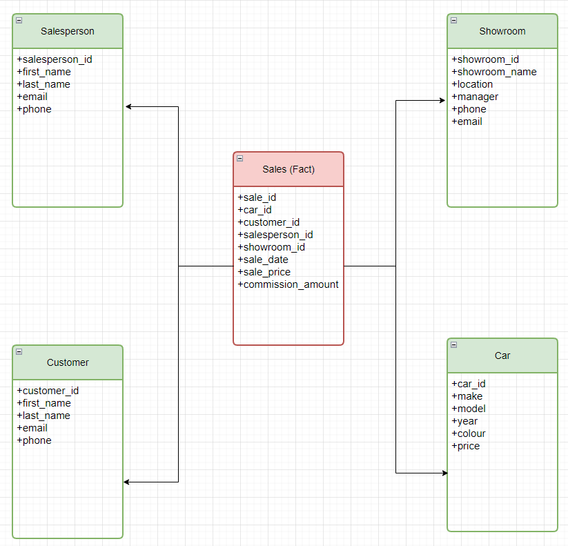
Applying the dimensional modeling approach to our example will result, as shown below, in a Sales fact table representing sales transactions with numeric measures (facts) and several dimension tables that provide the context for the facts with descriptive attributes.
- Data Vault
- Data Vaults organize data into three different types: hubs, links, and satellites
- Hubs represent core business entities. The primary key of Hub tables is usually derived by a combination of business concept ID, load date, and other metadata information
- Links represent relationships between hubs. It has only the join keys. It is like a Factless Fact table in the dimensional model. No attributes - just join keys
- Satellites store attributes about hubs or links. They have descriptive information on core business entities. They are similar to a normalized version of a Dimension table
- Data Vault is a “write-optimized” modeling style
- Great fit for data lakes and lakehouse approach
- Supports agile development approaches:
- It can be easily extended without massive refactoring like the dimensional models
- Additional hubs can be easily added to links and additional satellites can be added to a Hub with minimal changes
- Existing ETL jobs need significantly less refactoring when the data model changes
- Data Vaults organize data into three different types: hubs, links, and satellites
Modeling Techniques Implementation on Databricks Lakehouse Platform
A data Lakehouse is a new, open architecture that combines the best elements of data lakes and data warehouses. The Databricks Lakehouse is a large-scale enterprise-level platform that can host many use cases and data products. Therefore, it can support many different data modeling styles for different purposes and both normalized Data Vault (write-optimized) and denormalized dimensional models (read-optimized) data modeling styles have their place.
The application of both techniques can be especially recognized through the lenses of the Medallion Architecture.
The medallion architecture is a data design pattern used to logically organize data in a lakehouse, with the goal of incrementally and progressively improving the structure and quality of data as it flows through each layer of the architecture (from Bronze ⇒ Silver ⇒ Gold layer tables).
The following diagram summarizes the mapping of different layers, their purpose, and applied modeling techniques in each:
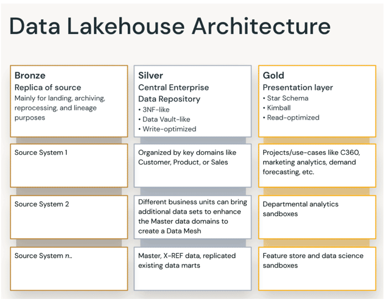
First data is landed in the Bronze layer in raw format using the same models of source systems in order to get converted to delta lake format. Next it flows into the Silver layer where it gets aggregated using more normalized model. Finally, the gold layer is meant for read-optimized presentation layer using denormalized models.
With this we have reached the end of this post, I hope you enjoyed it!
If you have any remarks or questions, please don’t hesitate and do drop a comment below.
Stay tuned!
Recap
In this article we covered the three main data warehouse modeling techniques and relevant design concepts and how they are applied in some form of combination taking the example of Databricks lakehouse platform.
Happy learning!
Resources
https://www.snowflake.com/guides/difference-between-data-warehouse-and-data-mart/